Mathematical Model of an IMU
If you don't know what an IMU is, I would recommend going through my
What is an IMU? tutorial .
Let us assume that our IMU is a 6-DoF one, i.e., it has a 3 axis gyro and a 3 axis acc. A 9-DoF IMU is commonly called MARG (Magnetic, Angular Rate and Gravity) sensor. A simple mathematical model of the gyro and acc is given below.
Gyroscope Model:
$$ \omega = \hat{\omega} + \mathbf{b}_g + \mathbf{n}_g $$
Here, \(\omega\) is the measured angular velocity from the gyro, \(\hat{\omega}\) is the latent ideal angular velocity we wish to recover, \(\mathbf{b}_g\) is the gyro bias which changes with time and other factors like temparature, \(\mathbf{n}_g\) is the white gaussian gyro noise.
The gyro bias is modelled as \(\mathbf{\dot{b}}_g = \mathbf{b}_{bg}(t) \sim \mathcal{N}(0, Q_g)\) where \(Q_g\) is the covariance matrix which models gyro noise.
Accelerometer Model:
$$ \mathbf{a} = R^T(\mathbf{\hat{a}} - \mathbf{g}) + \mathbf{b}_a + \mathbf{n}_a $$
Here, \(\mathbf{a}\) is the measured acceleration from the acc, \(\mathbf{\hat{a}}\) is the latent ideal acceleration we wish to recover, \(R\) is the orientation of the sensor in the world frame, \(\mathbf{g}\) is the acceleration due to gravity in the world frame, \(\mathbf{b}_a\) is the acc bias which changes with time and other factors like temparature, \(\mathbf{n}_a\) is the the white gaussian acc noise.
The acc bias is modelled as \(\mathbf{\dot{b}}_a = \mathbf{b}_{ba}(t) \sim \mathcal{N}(0, Q_a)\) where \(Q_a\) is the covariance matrix which models acc noise.
Here the orientation of the sensor is either known from external sources such as a motion capture system or a camera or estimated by sensor fusion.
Madgwick Filter
Before we start talking about the madgwick filter formulation, let us formally define coordinate axes we will use. Let the letters \(I, W, B\) denote inertial, world and body frames respectively. Generally \(B\) and \(I\) are the same but they don't have to be. A pre-subscript denotes the source coordinate frame and a pre-superscript denotes the destination coordinate frame. For eg., \({}^{B}_{A}X\) transforms \(X\) from coordinate frame \(A\) to \(B\). If only a pre-superscript is present, it means that the quantity was measured and is represented in the same coordinate frame represented by the pre-superscript.
The desired output is to estimate the attitude/angle/orientation of the IMU sensor in the world frame, i.e., estimating \({}^{W}_{I}\mathbf{q}\). We use \(\mathbf{q}\) to denote the orientation represented in the form of a
Quaternion. If you don't know much about quaternions, I would highly recommend to read
this Wikipedia article on quaternions.
The Mahony filter is a glorified [Complementary Filter](tutorials/attitudeest/imu) with significant improvements to accuracy without significant markup in computation time. Even today, it remains to be one of the most popular filters used in racing quadrotors where time is money.
The Madgwick filter formulates the attitude estimation problem in quaternion space. The general idea of the Madgwick filter is to estimate \({}^{I}_{W}\mathbf{q}_{t+1}\) by fusing/combining attitude estimates by integrating gyro measurements \({}^{I}_{W}\mathbf{q}_{\omega}\) and direction obtained by the accelerometer measurements. In essence, the gyro estimates of attitude are used as accurate depictions in a small amount of time and faster movements and the acc estimates of attitude are used as accurate directions to compensate for long term gyro drift by integration.
As in
Complementary Filter , the attitude is estimated from the gyro by numerical integration. The attitude estimation from the acc is done by using a gradient descent algorithm to solve the following minimzation problem.
$$
\min_{ {}^{I}_{W}\mathbf{\hat{q}} \in \mathbb{R}^{4 \times 1} } f\left({}^{I}_{W}\mathbf{\hat{q}}, {}^{W}\mathbf{\hat{g}}, {}^{I}\mathbf{\hat{a}} \right)
$$
$$
f\left({}^{I}_{W}\mathbf{\hat{q}}, {}^{W}\mathbf{\hat{g}}, {}^{I}\mathbf{\hat{a}} \right) = {}^{I}_{W}\mathbf{\hat{q^*}} \otimes {}^{W}\mathbf{\hat{g}} \otimes {}^{I}_{W}\mathbf{\hat{q}} - {}^{I}\mathbf{\hat{a}}
$$
Here, \(\mathbf{q}^*\) denotes the conjugate of \(\mathbf{q}\) and \(\otimes\) indicates quaternion multiplication. \({}^{W}\mathbf{\hat{g}}\) denotes the normalized gravity vector and is given by \({}^{W}\mathbf{\hat{g}} = \begin{bmatrix} 0 & 0 & 0 & 1\end{bmatrix}^T\) and \({}^{I}\mathbf{\hat{a}}\) denotes the normalized acc measurements. From now on \(\mathbf{\hat{x}}\) denotes normalized version of \(\mathbf{x}\).
Following are the steps for attitude estimation using a Madgwick filter (Refer to Fig. 1 shown below for an overview of the algorithm).
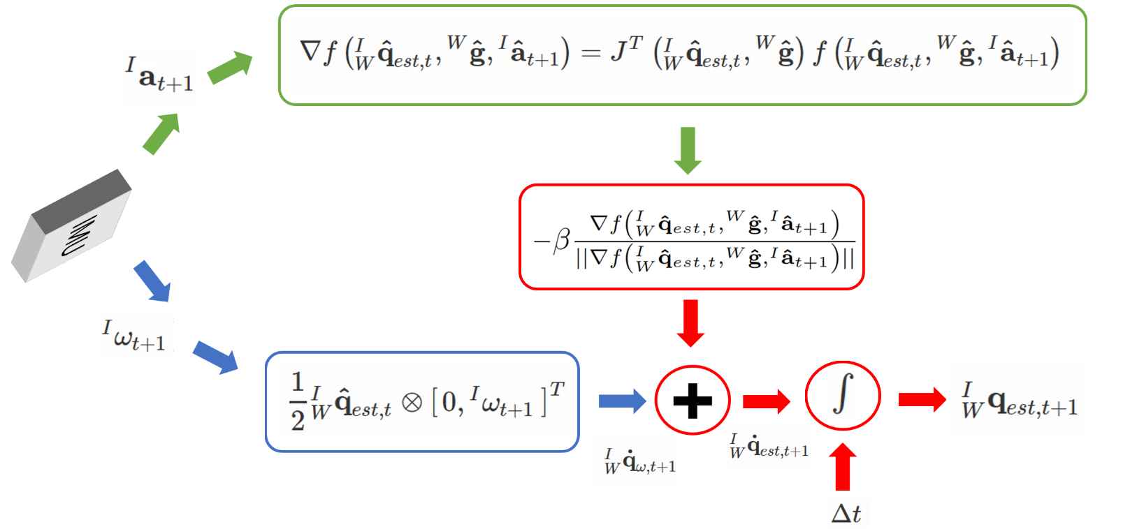
Fig 1: Overview of Madgwick Filter.
-
Step 1: Obtain sensor measurements
Obtain gyro and acc measurements from the sensor. Let \({}^I\omega_t\) and \({}^I\mathbf{a}_t\) denote the gyro and acc measurements respectively. Also, \({}^I\mathbf{\hat{a}}_t\) denotes the normalized acc measurements.
-
Step 2 (a): Orientation increment from Acc
Compute orientation increment from acc measurements (gradient step).
\( \nabla f\left( {}^{I}_{W}\mathbf{\hat{q}}_{est, t}, {}^{W}\mathbf{\hat{g}}, {}^{I}\mathbf{\hat{a}}_{t+1} \right) = J^T\left( {}^{I}_{W}\mathbf{\hat{q}}_{est, t}, {}^{W}\mathbf{\hat{g}} \right) f\left( {}^{I}_{W}\mathbf{\hat{q}}_{est, t}, {}^{W}\mathbf{\hat{g}}, {}^{I}\mathbf{\hat{a}}_{t+1} \right) \)
\( f\left( {}^{I}_{W}\mathbf{\hat{q}}_{est, t}, {}^{W}\mathbf{\hat{g}}, {}^{I}\mathbf{\hat{a}}_{t+1} \right) = \begin{bmatrix}
2\left( q_2q_4 - q_1q_3\right) - a_x\\
2\left( q_1q_2 + q_3q_4\right) - a_y\\
2\left( \frac{1}{2} - q_2^2 - q_3^2\right) - a_z\\
\end{bmatrix} \)
\( J\left( {}^{I}_{W}\mathbf{\hat{q}}_{est, t}, {}^{W}\mathbf{\hat{g}} \right) = \begin{bmatrix}
-2q_3 & 2q_4 & -2q_1 & 2q_2 \\
2q_2 & 2q_1 & 2q_4 & 2q_3 \\
0 & -4q_2 & -4q_3 & 0\\
\end{bmatrix} \)
Update Term (Attitude component from acc measurements) is given by
\(
{}^{I}_{W}\mathbf{q}_{\nabla, t+1} = - \beta\frac{\nabla f\left( {}^{I}_{W}\mathbf{\hat{q}}_{est, t}, {}^{W}\mathbf{\hat{g}}, {}^{I}\mathbf{\hat{a}}_{t+1} \right)}{\vert \vert \nabla f\left( {}^{I}_{W}\mathbf{\hat{q}}_{est, t}, {}^{W}\mathbf{\hat{g}}, {}^{I}\mathbf{\hat{a}}_{t+1} \right) \vert \vert}
\)
Look at green parts in Fig. 1.
Step 2 (b): Orientation increment from Gyro
Compute orientation increment from gyro measurements (numerical integration).
\(
{}^{I}_{W}\mathbf{\dot{q}}_{\omega,t+1} = \frac{1}{2} {}^{I}_{W}\mathbf{\hat{q}}_{est,t}\otimes \begin{bmatrix} 0, {}^{I}\omega_{t+1} \end{bmatrix}^T\)
Look at blue parts in Fig. 1.
Step 3: Fuse Measurements
Fuse the measurments from both the acc and gyro to obtain the estimated attitude \( {}^{I}_{W}\mathbf{\hat{q}}_{est, t+1}\).
\(
{}^{I}_{W}\mathbf{\dot{q}}_{est, t+1} = {}^{I}_{W}\mathbf{\dot{q}}_{\omega, t+1} + {}^{I}_{W}\mathbf{q}_{\nabla, t+1}
\)
\( {}^{I}_{W}\mathbf{q}_{est, t+1} = {}^{I}_{W}\mathbf{\hat{q}}_{est, t} + {}^{I}_{W}\mathbf{\dot{q}}_{est, t+1} \Delta t
\)
Here, \(\Delta t\) is the time elapsed between two samples at \(t\) and \(t+1\). Look at red parts in Fig. 1.
Repeat steps 1 to 3 for every time instant.
In a Madgwick filter, the only tunable parameter is trade off parameter \(\beta\) which determines when the gyro has to take over the acc. Also, the user needs to specify the initial estimates of the attitude, biases and sampling time. The initial attitude can be assumed to be zero if th device is at rest or it has to be obtained by external sources such as a motion capture system or a camera. The bias is computed by taking an average of samples with the IMU at rest and computing the mean value. Note that this bias changes over time and the filter will start to drift over time. The sampling time is the inverse of the operating frequency of the IMU and is specified generally at the driver level.
References